Circle: Least Squares Fit
Documentation Plus Sample Code
This is a very easy and very accurate algorithm for correcting hard iron errors in a magnetic compass. It uses all your data points to come up with a least-squares error fit. It is much better than the pencil and paper method that uses only four points (min and max on x and y coordinates) and throws all the rest away.
Least Squares Algorithms
- Circle: Quick, easy solution to simple 2D hard iron problem
- Sphere: Quick, easy solution to simple 3D hard iron problem
- Ellipse: 2D Hard and Soft iron solution
- Ellipsoid: 3D Hard and Soft iron solution
- Precision Ellipsoid: Precision Iterative 3D Hard and Soft iron solution
Algorithm
The classic equation for a circle centered at a,b with radius R is:
( x - a )2 + ( y - b )2 = R2
We can rearrange this to a form more suitable for a solution by rewriting it as:
A (x2 + y2) + B x + C y = 1
Suppose now that we have n noisy input samples of each component x and y; n >= 3. More than the minimum
number of points are taken in order to prevent a small number of bad samples from seriously biasing the results.
Similarly, the samples are distributed around the circle to keep the solution from bulging out one
side or the other.
We can form the J matrix, an
n-row by 3-column matrix. The ith row of this matrix is
[(xi2 + yi2) , xi , yi ]
So, for example, if the ith data point were at (3,2) then the ith row
of the J matrix would be [(32+22),3,2] = [13,3,2].
Now collect the coefficients
A, B, and C into a column vector ABC, and we can write the n equations as
J ABC = K
where K is a column of ones. The J matrix is usually not square, so we cannot take its inverse. A modification of the equation makes it more inverse-friendly. Multiply both sides by the transpose of J. This creates a square matrix. We take the inverse of that matrix and multiply both sides by it. The resulting equation is
( JTJ )-1 JTJ ABC =( JTJ )-1 JT K
ABC =( JTJ )-1 JT K
Everything on the right is known. So, we just form the matrices, take the indicated inverse, and multiply the matrices out. The output vector, ABC, has the components
A = ABC[0]
B = ABC[1]
C = ABC[2]
We convert back to standard form using
a = xofs = -B/(2 A)
b = yofs = -C/(2 A)
R = sqrt(4 A + B2 + C2)/(2 A)
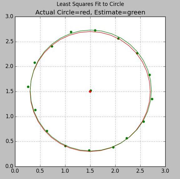
Least Squares Fit to Circle using Noisy Samples
Python Source Code ls_circle.py
Inputs are two NumPy arrays for the observed x and y coordinates
Output is the tuple (X,Y,R) where X,Y is the center and R is the radius
#least squares fit to a circle

import numpy as np

def ls_circle(xx,yy):
   asize = np.size(xx)
   print 'Circle input size is ' + str(asize)
   J=np.zeros((asize,3))
   ABC=np.zeros(asize)
   K=np.zeros(asize)

   for ix in range(0,asize):
      x=xx[ix]
      y=yy[ix]

      J[ix,0]=x*x + y*y;
      J[ix,1]=x;
      J[ix,2]=y;
      K[ix]=1.0

   K=K.transpose()
   JT=J.transpose()
   JTJ = np.dot(JT,J)
   InvJTJ=np.linalg.inv(JTJ);

   ABC= np.dot(InvJTJ, np.dot(JT,K))
   #If A is negative, R will be negative
   A=ABC[0]
   B=ABC[1]
   C=ABC[2]

   xofs=-B/(2*A)
   yofs=-C/(2*A)
   R=np.sqrt(4*A + B*B + C*C)/(2*A)
   if R < 0.0: R = -R
   return (xofs,yofs,R)


if __name__ == '__main__':
# Test of least squares fit to a circle
# Samples have random noise added to both X and Y components
# True center is at (1.5, 1.5); true radius is 1.2

# Output:
# Circle input size is 16
# Center at (  1.5130,  1.5204) Radius:  1.2097

   xx = np.array(
[ 2.2331,   2.5712,   2.7397,   2.6899,
  2.4360,   2.0610,   1.5977,   1.1202,
  0.7375,   0.3965,   0.2624,   0.4069,
  0.6400,   1.0078,   1.4793,   1.9598])

   yy = np.array (
[ 0.5676,   0.9002,   1.3492,   1.8300,
  2.2661,   2.5607,   2.7243,   2.6918,
  2.4032,   2.0740,   1.5964,   1.1327,
  0.7084,   0.4101,   0.3221,   0.3840])
   ans = ls_circle(xx,yy)
   ss="Center at (%8.4f,%8.4f) Radius:%8.4f" % ans
   print ss
MATLAB / Octave Source Code ls_circle.m
First two columns of input matrix are the observed x and y coordinates
Output is similar to the python code. Note that in Python an index starts at zero while MATLAB starts at 1
function [xofs,yofs,R]=ls_circle(inmat)

   [rr,cc]=size(inmat);
   J=zeros(rr,3);
   ABC=zeros(rr,3);

   XX=inmat(:,1);
   YY=inmat(:,2);

   for iloop=1:rr
      x=XX(iloop);
      y=YY(iloop);
      K(iloop)=1;
      J(iloop,1)=x*x + y*y;
      J(iloop,2)=x;
      J(iloop,3)=y;
   end
   K=K';
   JT=J';
   JTJ = JT*J;
   InvJTJ=inv(JTJ);

   ABC= InvJTJ*JT*K;
   A=ABC(1);
   B=ABC(2);
   C=ABC(3);
   xofs=-B/(2*A);
   yofs=-C/(2*A);
   R=sqrt(4*A + B*B + C*C)/(2*A);

return;
©2022 Tom Judd
www.juddzone.com
Carlsbad, CA
USA