Fit data points to an Ellipse

Documentation Plus Sample Code

Given a set of points, find the ellipse that best fits the points in a least squares sense

Least Squares Algorithms

Circle: Quick, easy solution to simple 2D hard iron problem
Sphere: Quick, easy solution to simple 3D hard iron problem
Ellipse: 2D Hard and Soft iron solution
Ellipsoid: 3D Hard and Soft iron solution
Precision Ellipsoid: Precision Iterative 3D Hard and Soft iron solution

Algorithm

The standard high school equation for an ellipse centered at a,b with major and minor axes A and B is:

( x - a )²/A² + ( y - b )²/B² = 1

This is not the most general form. But it is what you get if you try to search for an equation on the internet. A more general ellipse can be tilted, so that the bulgy part is NOT aligned with one of the axes. In order tilt the ellipse we have to throw in an xy term. We can write the equation as:

A x² + B x y + C y² + D x + E y = 1

A x² + B x y + C y² + D x + E y - 1 = 0

or if we multiply through by some arbitrary constant

A x² + B x y + C y² + D x + E y + F = 0

There are only five independent parameters: two to define the center, two to define the major and minor axes, and one to define the tilt angle. We have six in the last equation. The extra parameter 'F' is just a scaled version of '1'. It is convenient to express it this way so the coefficients can be normalized (sum of their squares equals 1)

Suppose now that we take n noisy input samples of each component x and y; n >= 5. Two rules are critical to follow when taking data points:

Oversample the data. More than the minimum number of points is taken so that a few bad points do not bias the solution
Distribute the samples all around the ellipse. Bunching samples on one side of the ellipse leaves the solution unconstrained on the other side. You then allow the solution to bulge or contract on that side

We can form the J matrix, an n-row by 5-column matrix. The i^th row of this matrix is

[x_i², x_i y_i , y_i² , x_i , y_i ]

So, for example, if the i^th data point were at (3,2) then the i^th row of the J matrix would be [(3², 3*2, 2²,3,2] = [9,6,4,3,2].
Now collect the coefficients A, B, C, D, and E into a column vector ABC, and we can write the n equations as

J ABC = K

where K is a column of ones. The J matrix is usually not square, so we cannot take its inverse. A modification of the equation makes it more inverse-friendly. Multiply both sides by the transpose of J. This creates a square matrix. We take the inverse of that matrix and multiply both sides by it. The resulting equation is

( J^TJ )^-1 J^TJ ABC =( J^TJ )^-1 J^T K

ABC =( J^TJ )^-1 J^T K

Everything on the right is known. So, we just form the matrices, take the indicated inverse, and multiply the matrices out. The output vector, ABC, has the components

A..E = ABC[0]..ABC[4]

We bring the 1 to the other side of the equation and so get

A..F = ABC[0]..ABC[5]

The 'F' term is -1.

We are not done yet. We have an answer but it is not in an easily understandable form. From the polynomial coefficients we have to obtain the center of the ellipse, the major and minor axes, and the tilt. The function that does this is polyToParams. The listing shows that we first convert the polynomial to algebraic form such that

X^T Amat X

regenerates the polynomial. Notice the division by two in the listing for all the off diagonal elements. Sometimes the factor of two is pre-included in the polynomial, e.g. instead of a Dx term, it is 2Dx term..

The center of the ellipse requires the use of the inverse of a matrix, while the axes and rotation matrix are obtained by the eigenvalues and eigenvectors of a matrix. This may seem a bit odd. Once we have the answer, we have to solve it again to get the answer we want. Later on we will find a way to skip over the polynomial step and go directly to the parameter form.

The final listing is the sample output using the noisy x and y values in the source. It will be useful if you want to convert to C or another programming language.

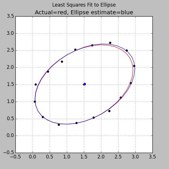
Least Squares Fit to Ellipse using Noisy Samples

Python Source Code ls_ellipse.py

Inputs are two NumPy arrays for the observed x and y coordinates

Output is a vector of the polynomial coefficients. The listing includes two sets of test data. The first is noise free, the second has added noise. It is the sample in the plot.


import numpy as np

#least squares fit to an ellipse
# A x^2 + B xy + C y^2 + Dx + Ey = 1
#
# Returns coefficients A..F
# A x^2 + B xy + C y^2 + Dx + Ey + F = 0
# where F = -1

def ls_ellipse(xx,yy):

   # change xx from vector of length N to Nx1 matrix so we can use hstack
   x = xx[:,np.newaxis]
   y = yy[:,np.newaxis]

   J = np.hstack((x*x, x*y, y*y, x, y))
   K = np.ones_like(x) #column of ones

   JT=J.transpose()
   JTJ = np.dot(JT,J)
   InvJTJ=np.linalg.inv(JTJ);
   ABC= np.dot(InvJTJ, np.dot(JT,K))

   # ABC has polynomial coefficients A..E
   # Move the 1 to the other side and return A..F
   # A x^2 + B xy + C y^2 + Dx + Ey - 1 = 0
   eansa=np.append(ABC,-1)

   return eansa


if __name__ == '__main__':

# Test of least squares fit to an ellipse
# Samples have random noise added to both X and Y components
# True center is at (1.5, 1.5);
# X axis is 1.55, Y axis is 1.0, tilt is 30 degrees
# (or -150 from symmetry)
#
# Polynomial coefficients, F term is -1:
# A x^2 + B xy + C y^2 + Dx + Ey - 1 = 0
#
# A= -0.53968362, B=  0.50979868, C= -0.8285294
# D=  0.87914926, E=  1.72765849, F= -1

# Polynomial coefficients after normalization:
# A x^2 + B xy + C y^2 + Dx + Ey + F = 0
#
# A=  0.22041087, B= -0.20820563, C=  0.33837767
# D= -0.3590512,  E= -0.70558878  F=  0.40840756

# Test data, no noise
   x0 = np.array(
[ 2.2255,   2.5995,   2.8634,   2.9163,
  2.6252,   2.1366,   1.6252,   1.1421,
  0.7084,   0.3479,   0.1094,   0.1072,
  0.4497,   0.9500,   1.4583,   1.9341])

   y0 = np.array(
[ 0.7817,   1.1319,   1.5717,   2.0812,
  2.5027,   2.6578,   2.6150,   2.4418,
  2.1675,   1.8020,   1.3480,   0.8351,
  0.4534,   0.3381,   0.4061,   0.5973])

# Test data with added noise
   xnoisy = np.array(
[ 2.2422,   2.5713,   2.8677,   2.9708,
  2.7462,   2.2695,   1.7423,   1.2501,
  0.8562,   0.4489,   0.0933,   0.0639,
  0.3024,   0.7666,   1.2813,   1.7860])

   ynoisy = np.array(
[ 0.7216,   1.1190,   1.5447,   2.0398,
  2.4942,   2.7168,   2.6496,   2.5163,
  2.1730,   1.8725,   1.5018,   0.9970,
  0.5509,   0.3211,   0.3729,   0.5340])


   print '\n=============================='
   print '\nSolution for Perfect Data (to 4 decimal places)'

   ans0= ls_ellipse(x0,y0)
   printAns(ans0,x0,y0,0)

   print '\n=============================='
   print '\nSolution for Noisy Data'

   ans = ls_ellipse(xnoisy,ynoisy)
   printAns(ans,xnoisy,ynoisy,0)

Helper functions to convert the polynomial output into user-friendly parameters (center, axis lengths, tilt) are below. The first is polyToParams. It takes the polynomial output and turns it into user-understandable parameters: the center, major and minor axes, and the tilt angle in degrees. It also returns the rotation matrix that can be used to validate the ellipse. The second function is printAns. It presents the parameters in useful form. It also shows you how to use the rotation matrix to check your answer. The output for the noisy data set is in the final listing

from numpy.linalg import eig, inv
def polyToParams(v,printMe):

   # convert the polynomial form of the ellipse to parameters
   # center, axes, and tilt
   # v is the vector whose elements are the polynomial
   # coefficients A..F
   # returns (center, axes, tilt degrees, rotation matrix)

   #Algebraic form: X.T * Amat * X --> polynomial form

   Amat = np.array(
   [
   [v[0],     v[1]/2.0, v[3]/2.0],
   [v[1]/2.0, v[2],     v[4]/2.0],
   [v[3]/2.0, v[4]/2.0, v[5]    ]
   ])

   if printMe: print '\nAlgebraic form of polynomial\n',Amat

   #See B.Bartoni, Preprint SMU-HEP-10-14 Multi-dimensional Ellipsoidal Fitting
   # equation 20 for the following method for finding the center
   A2=Amat[0:2,0:2]
   A2Inv=inv(A2)
   ofs=v[3:5]/2.0
   cc = -np.dot(A2Inv,ofs)
   if printMe: print '\nCenter at:',cc

   # Center the ellipse at the origin
   Tofs=np.eye(3)
   Tofs[2,0:2]=cc
   R = np.dot(Tofs,np.dot(Amat,Tofs.T))
   if printMe: print '\nAlgebraic form translated to center\n',R,'\n'

   R2=R[0:2,0:2]
   s1=-R[2, 2]
   RS=R2/s1
   (el,ec)=eig(RS)

   recip=1.0/np.abs(el)
   axes=np.sqrt(recip)
   if printMe: print '\nAxes are\n',axes  ,'\n'

   rads=np.arctan2(ec[1,0],ec[0,0])
   deg=np.degrees(rads) #convert radians to degrees (r2d=180.0/np.pi)
   if printMe: print 'Rotation is ',deg,'\n'

   inve=inv(ec) #inverse is actually the transpose here
   if printMe: print '\nRotation matrix\n',inve
   return (cc[0],cc[1],axes[0],axes[1],deg,inve)



   def printAns(pv,xin,yin,verbose):
      print '\nPolynomial coefficients, F term is -1:\n',pv

      #normalize and make first term positive
      nrm=np.sqrt(np.dot(pv,pv))
      enrm=pv/nrm
      if enrm[0] < 0.0:
         enrm = - enrm
      print '\nNormalized Polynomial Coefficients:\n',enrm

      #convert polynomial coefficients to parameterized ellipse (center, axes, and tilt)
      #also returns rotation matrix in last parameter
      # either pv or normalized parameter will work
      # params = polyToParams(enrm,verbose)

      params = polyToParams(pv,verbose)

      print "\nCenter at  %10.4f,%10.4f (truth is 1.5,  1.5)" % (params[0],params[1])
      print "Axes gains %10.4f,%10.4f (truth is 1.55, 1.0)" % (params[2],params[3])
      print "Tilt Degrees %10.4f (truth is 30.0)" % (params[4])

      R=params[5]
      print '\nRotation Matrix\n',R

      # Check solution
      # Convert to unit sphere centered at origin
      #  1) Subtract off center
      #  2) Rotate points so bulges are aligned with x, y axes (no xy term)
      #  3) Scale the points by the inverse of the axes gains
      #  4) Back rotate
      # Rotations and gains are collected into single transformation matrix M

      # subtract the offset so ellipse is centered at origin
      xc=xin-params[0]
      yc=yin-params[1]

      # create transformation matrix
      L = np.diag([1/params[2],1/params[3]])
      M=np.dot(R.T,np.dot(L,R))
      print '\nTransformation Matrix\n',M

      # apply the transformation matrix
      [xm,ym]=np.dot(M,[xc,yc])
      # Calculate distance from origin for each point (ideal = 1.0)
      rm = np.sqrt(xm*xm + ym*ym)

      print "\nAverage Radius  %10.4f (truth is 1.0)" % (np.mean(rm))
      print "Stdev of Radius %10.4f " % (np.std(rm))


Solution for Noisy Data

Polynomial coefficients, F term is -1:
[-0.53968362  0.50979868 -0.8285294   0.87914926  1.72765849 -1.        ]

Normalized Polynomial Coefficients:
[ 0.22041087 -0.20820563  0.33837767 -0.3590512  -0.70558878  0.40840756]

Center at      1.5291,    1.5130 (truth is 1.5,  1.5)
Axes gains     1.5822,    1.0011 (truth is 1.55, 1.0)
Tilt Degrees  -149.7677 (truth is 30.0)

Rotation Matrix
[[-0.86399095 -0.50350734]
 [ 0.50350734 -0.86399095]]

Transformation Matrix
[[ 0.72503804 -0.15961178]
 [-0.15961178  0.90590626]]

Average Radius      1.0015 (truth is 1.0)
Stdev of Radius     0.0321

Notice the difference between the truth tilt (30) and the calculated tilt (~-150). Tilts were obtained from the transformation matrix. From symmetry, these two are the same