Precision 3D Compass Calibration
Iterative Solutions -- Shortcut Calibration -- Sample Code
The advantage of the precision iterative solution presented here is that it can be configured to incorporate different constraints without rewriting the whole code. In particular, I show how to include accelerometer information. This is essential for high precision compasses. Compare the function radiusErr which uses only magnetometer data with magDotAccErr which includes accelerometer info
Least Squares Algorithms
- Circle: Quick, easy solution to simple 2D hard iron problem
- Sphere: Quick, easy solution to simple 3D hard iron problem
- Ellipse: 2D Hard and Soft iron solution
- Ellipsoid: 3D Hard and Soft iron solution
- Precision Ellipsoid: Precision Iterative 3D Hard and Soft iron solution
Compass Calibration Code for Iterative Precision Calibration
Unzip to a directory. Run the batch file (runcal3.bat) in Windows, or the bash script (runcal3.sh) in Linux. Source is Python 3.
Two Python source files are included:
- gendat3.py This code generates test data: samples of the magnetic field with known errors.
It also produces a set of samples at known azimuths around a circle. Compass accuracy can be computed after
correcting for anomalies.
Command line parameters allow you to completely specify the position, orientation, and shape of the ellipsoid sample envelope. You can also add noise and asymmetry. See the code for suggested real-world values.
-
itermag3.py This code takes the sample points and tries to correct for the errors using two
different techniques: a symmetric iteration, so called because the 3x3 transformation matrix is symmetric,
and a precision iteration technique which allows the off diagonal elements to converge independently.
If no command line parameters are given, then hard-coded samples are used. Otherwise, you can specify an input file that contains the output from the above data generator.
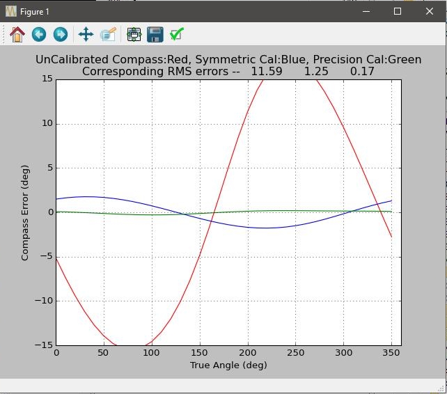
Truth and calculated offset and transformation matrix are displayed for comparison. You also get an estimated final compass accuracy expressed in degrees. Finally, I plot the compass error as a function of the direction both before and after calibrations.
Sample Output
Classic Calibration
The classic method for calibrating a 3D compass is to first solve for the ellipsoid that best fits the data samples. This involves solving a polynomial with nine degrees of freedom. Once found, the center, axes lengths, and orientation are determined. From these we can get the offset and transformation matrix that fully correct the data points.
Classic 3D Compass Calibration Process
- Solve for the polynomial coefficients of a 3D ellipsoid e.g.
A x2 + B y2 + C z2 + D x y + E x z + F y z + G x + H y + I z = 1
Each observed data point provides one set of x, y, and z for the equation. With nine unknowns, we need at least nine well placed data points to solve for the coefficients. - Solve for the center of the ellipsoid from the solution.
- Subtract the center from the solution (offsets px,py,pz in the diagram). This moves the ellipsoid to the origin of our coordinate system
- Solve for the eigenvalues and eigenvectors of the centered ellipsoid. The eigenvalues are the axis gains. The eigenvectors form a rotation matrix which defines the orientation of the ellipsoid
- Form the transformation matrix T from the gains G and orientation matrix R:
T = RT (A G-1/2 ) R
where A is a normalization constant and G-1/2 is a diagonal matrix whose elements are the recipricol square roots of the gains. The transformation matrix plus the offsets when applied to the observed data, will correct for the perturbations that generated the ellipsoid. Note that you have to subtract the offsets first before applying any rotation.
Shortcut Calibration
When I looked at the classic process for compass calibration I thought it was too much work. I thought development would be quicker if I skipped all the intermediate stuff and focused on getting the offsets and transformation matrix via an iterative process. The steps are fewer and the math is simpler, so there is less opportunity for a mistake. Iterative solutions can be slow; but I thought it best to follow an old development maxim:
Get it to work; then get it to work fast.
So, that's what I did.
Tom's 3D Compass Calibration Shortcut
- Solve iteratively for the offsets and transformation matrix.
Iterative Solutions
The normal constraint used for compass calibration is that the length of the magnetic field vector should be constant in any orientation. But the resulting solutions have only nine parameters, sufficient for three offsets and six elements of a symmetric transformation matrix. Adding tighter constraints enables one to obtain a twelve-parameter asymmetric solution; three offsets plus all nine elements of the transformation matrix contribute to the solution. The simplest constraint that mixes in the accelerometer data with the magnetometer data is that the dot product of the two is constant
If x, y, and z are the components of the magnetic field before applying the corrections, then we have
xp = [ A11( x - Ox) + A12( y - Oy) + A13( z - Oz)]
yp = [ A21( x - Ox) + A22( y - Oy) + A23( z - Oz)]
zp = [ A31( x - Ox) + A32( y - Oy) + A33( z - Oz)]
where xp, yp, and zp are the components after the transformation. Offsets are Ox,Oy,and Oz and the transformation matrix has the elements A11...A33. In terms of our twelve parameters the offsets are p0 through p2 and the transformation matrix is built row by row from the remaining nine: p3 through p11.The dot product between the mag and accel fields for a single sample is
Fi = xpax + ypay + zpaz =
[ A11( x - Ox) + A12( y - Oy) + A13( z - Oz)]ax +
[ A21( x - Ox) + A22( y - Oy) + A23( z - Oz)]ay +
[ A31( x - Ox) + A32( y - Oy) + A33( z - Oz)]az
Our constraint is that the dot product be constant, e.g. Fc. The dot product for our current set of components is Fi. We can postulate that if we changed the parameters (offset and transformation matrix) in the right way then we can get our sample estimate Fi to match the actual Fc:
Fc = Fi + (∂Fi/∂p0) Δp0 + ... + (∂Fi/∂p11) Δp11
The Error between the two is Ei = Fc - Fi
We can calculate the error for each sample point and the derivatives for each point, and so form the matrix equation
E = D Δp
These equations are solved in a manner similar to the other least squares fits, except that the output is a set of changes to the parameters that, for each step in the iteration, brings the parameters closer to the optimal solution
Δp =( DTD )-1 DT E
The analytic form of the partial derivative is relatively simple for the dot product. First the offsets as shown with Ox. It occurs in three places in the above equation for Fi. By inspection we can write the derivative as
∂Fi/∂Ox = - [ A11ax + A21ay + A31az ]
In the code it is written as
slopeArr[0]= -(params[3]*acc[0] + params[ 4]*acc[1] + params[ 5]*acc[2])
The equation for the matrix parameters is easier yet, because each matrix element appears in only one place. So for example we can write
∂Fi/∂A11 = (x - Ox)ax
In the code it is written as
slopeArr[3]= (mag[0]-params[0])*acc[0]
We obtain the partial derivatives for each sample point and form the D matrix. Going through the pseudo-inverse we can then solve for the deltas. The corrections are added to the current parameters. In the code look for the line:
p2=params + deltas
Notice we do not immediately update our working parameters. We first calculate the sigma. It should be improving (getting smaller). If it is not then you may want to do something about it. The usual problem is bad data. For example, in mobile applications there may be physical limitations to collecting a thorough set of 3D data. Car-mounted or person-mounted sensors may not usually be turned upside down. Data samples may fully cover the horizontal plane, but be otherwise sparse. Another problem is starting the iterations far from the solution. I have found that the iterations start to diverge if the initial point is further than about a third of the magnetic field from the solution. Therefore, starting with a good guess of the offsets is important. I have used the average of the samples as a starting point. Also, an estimate of the best sphere that matches the data will get you within striking distance. In the sample code, I used an ellipsoid approximation to obtain the center.
We also pause at this point to see if we are done. If the error is not getting any smaller then maybe it is time to stop. I usually have a convergence criterion AND an upper limit to the iterations to end the processing.
We can't solve for the change in the parameters just once and leave it there. Our linearization of the problem is an approximation to a non-linear problem. We generally need to reload the state with the new (better) parameters and re-solve the equations. We do this until our answer converges on the best fit solution.
Iterative Solutions with no Accelerometer Data
Precise accelerometer data is required for precision calibrations. That is not always possible, especially on a moving platform. So, I have included the code for two cases. The first, ellipsoid_iterate, makes use of both magnetometer and accelerometer data. The second, ellipsoid_iterate_symmetric, uses only magnetometer data. The output is the same for both: three offsets and a transformation matrix. The difference is that without the accelerometer data we get only six unique elements in the transformation matrix.
The final listing has the input and output for the two cases. For comparisons I have normalized the output matrices so that the first diagonal element is 1. You can see the difference in the output listing. The first off-diagonal elements in the asymmetric case are -0.1457 and -0.1647. In the symmetric case they are both -0.1518.
Python Source Code
Below are functions that implement the partial derivatives in the text. The first is the error function magDotAccErr . It takes the input magnetic vector components, transforms them with the parameters, then dots them into the acceleration vector. The difference from the nominal value (mdg) is returned as the error.
The next two functions are the analytical and numeric versions of the partial derivatives. Each function works. You can use one to check the other. We do not call magDotAccErr directly when using the numeric partials, because we want to allow for alternate error functions. The numeric version calls a generic errFn which calls another function depending on the mode. Current modes are
- 0 = Use constant radius as a constraint. Solve for nine parameters and a symmetric transformation matrix. Error function is radiusErr
- 1 = Use constant mag-accel dot product. Solve for twelve parameters and an asymmetric transformation matrix. Error function is magDotAccErr
def magDotAccErr(mag,acc,mdg,params):
   #offset and transformation matrix from parameters
   ofs=params[0:3]
   mat=np.reshape(params[3:12],(3,3))
   #subtract offset, then apply transformation matrix
   mc=mag-ofs
   mm=np.dot(mat,mc)
   #calculate dot product from corrected mags
   mdg1=np.dot(mm,acc)
   err=mdg-mdg1
   return err


def analyticPartialRow(mag,acc,target,params):
   err0=magDotAccErr(mag,acc,target,params)
   # ll=len(params)
   slopeArr=np.zeros(12)
   slopeArr[0]=  -(params[3]*acc[0] + params[ 4]*acc[1] + params[ 5]*acc[2])
   slopeArr[1]=  -(params[6]*acc[0] + params[ 7]*acc[1] + params[ 8]*acc[2])
   slopeArr[2]=  -(params[9]*acc[0] + params[10]*acc[1] + params[11]*acc[2])

   slopeArr[ 3]= (mag[0]-params[0])*acc[0]
   slopeArr[ 4]= (mag[1]-params[1])*acc[0]
   slopeArr[ 5]= (mag[2]-params[2])*acc[0]

   slopeArr[ 6]= (mag[0]-params[0])*acc[1]
   slopeArr[ 7]= (mag[1]-params[1])*acc[1]
   slopeArr[ 8]= (mag[2]-params[2])*acc[1]

   slopeArr[ 9]= (mag[0]-params[0])*acc[2]
   slopeArr[10]= (mag[1]-params[1])*acc[2]
   slopeArr[11]= (mag[2]-params[2])*acc[2]

   return (err0,slopeArr)

def numericPartialRow(mag,acc,target,params,step,mode):

   err0=errFn(mag,acc,target,params,mode)

   ll=len(params)
   slopeArr=np.zeros(ll)

   for ix in range(ll):

      params[ix]=params[ix]+step[ix]
      errA=errFn(mag,acc,target,params,mode)
      params[ix]=params[ix]-2.0*step[ix]
      errB=errFn(mag,acc,target,params,mode)
      params[ix]=params[ix]+step[ix]
      slope=(errB-errA)/(2.0*step[ix])
      slopeArr[ix]=slope

   return (err0,slopeArr)


def errFn(mag,acc,target,params,mode):
   if mode == 1: return magDotAccErr(mag,acc,target,params)
   return radiusErr(mag,target,params)

def radiusErr(mag,target,params):
   #offset and transformation matrix from parameters
   (ofs,mat)=param9toOfsMat(params)

   #subtract offset, then apply transformation matrix
   mc=mag-ofs
   mm=np.dot(mat,mc)

   radius = np.sqrt(mm[0]*mm[0] +mm[1]*mm[1] + mm[2]*mm[2] )
   err=target-radius
   return err
The next code snippet shows the actual iteration loop. Two versions are given, so scroll down to see them both. The first one is the precision solution with twelve parameters. The second fits nine parameters to the data using a milder constraint. I removed the comments in the second to give it a cleaner look. But you can get the general features of the code from the first.
ellipsoid_iterate
Precision calibration: uses both magnetometer and accelerometer data. Solves for 12 parameters, 3 offsets and 9 elements of a 3x3 transformation matrix.
# =============================

def ellipsoid_iterate(mag,accel,verbose):

   magCorrected=copy.deepcopy(mag)
   # Obtain an estimate of the center and radius
   # For an ellipse we estimate the radius to be the average distance
   # of all data points to the center
   (centerE,magR,magSTD)=ellipsoid_estimate2(mag,verbose)

   #Work with normalized data
   magScaled=mag/magR
   centerScaled = centerE/magR

   (accNorm,accR)=normalize3(accel)

   params=np.zeros(12)
   #Use the estimated offsets, but our transformation matrix is unity
   params[0:3]=centerScaled
   mat=np.eye(3)
   params[3:12]=np.reshape(mat,(1,9))

   #initial dot based on centered mag, scaled with average radius
   magCorrected=applyParams12(magScaled,params)
   (avgDot,stdDot)=mgDot(magCorrected,accNorm)

   nSamples=len(magScaled)
   sigma = errorEstimate(magScaled,accNorm,avgDot,params)
   if verbose: print 'Initial Sigma',sigma

   # pre allocate the data.  We do not actually need the entire
   # D matrix if we calculate DTD (a 12x12 matrix) within the sample loop
   # Also DTE (dimension 12) can be calculated on the fly.

   D=np.zeros([nSamples,12])
   E=np.zeros(nSamples)

   #If numeric derivatives are used, this step size works with normalized data.
   step=np.ones(12)
   step/=5000

   #Fixed number of iterations for testing.  In production you check for convergence

   nLoops=5

   for iloop in range(nLoops):
      # Numeric or analytic partials each give the same answer
      for ix in range(nSamples):
         #(f0,pdiff)=numericPartialRow(magScaled[ix],accNorm[ix],avgDot,params,step,1)
         (f0,pdiff)=analyticPartialRow(magScaled[ix],accNorm[ix],avgDot,params)
         E[ix]=f0
         D[ix]=pdiff
      #Use the pseudo-inverse
      DT=D.T
      DTD=np.dot(DT,D)
      DTE=np.dot(DT,E)
      invDTD=inv(DTD)
      deltas=np.dot(invDTD,DTE)


      p2=params + deltas

      sigma = errorEstimate(magScaled,accNorm,avgDot,p2)

      # add some checking here on the behavior of sigma from loop to loop
      # if satisfied, use the new set of parameters for the next iteration

      params=p2

      # recalculste gain (magR) and target dot product
      magCorrected=applyParams12(magScaled,params)
      (mc,mcR)=normalize3(magCorrected)
      (avgDot,stdDot)=mgDot(mc,accNorm)
      magR *= mcR
      magScaled=mag/magR

      if verbose:
         print 'iloop',iloop,'sigma',sigma

   return (params,magR)


# =============================
ellipsoid_iterate_symmetric
Symmetric calibration: uses only magnetometer data. Solves for 9 parameters, 3 offsets and 6 elements of a symmetric 3x3 transformation matrix.
# =============================

def ellipsoid_iterate_symmetric(mag,verbose):

   (centerE,magR,magSTD)=ellipsoid_estimate2(mag,0)

   magScaled=mag/magR
   centerScaled = centerE/magR

   params9=np.zeros(9)
   ofs=np.zeros(3)
   mat=np.eye(3)
   params9=ofsMatToParam9(centerScaled,mat,params9)

   nSamples=len(magScaled)
   sigma = errorEstimateSymmetric(magScaled,1,params9)
   if verbose: print 'Initial Sigma',sigma

   step=np.ones(9)
   step/=5000
   D=np.zeros([nSamples,9])
   E=np.zeros(nSamples)
   nLoops=5

   for iloop in range(nLoops):

      for ix in range(nSamples):
         (f0,pdiff)=numericPartialRow(magScaled[ix],magScaled[ix],1,params9,step,0)
         E[ix]=f0
         D[ix]=pdiff
      DT=D.T
      DTD=np.dot(DT,D)
      DTE=np.dot(DT,E)
      invDTD=inv(DTD)
      deltas=np.dot(invDTD,DTE)

      p2=params9 + deltas

      (ofs,mat)=param9toOfsMat(p2)
      sigma = errorEstimateSymmetric(magScaled,1,p2)

      params9=p2

      if verbose:
         print 'iloop',iloop,'sigma',sigma

   return (params9,magR)

# =============================
The next code snippet demonstrates how to call the ellipsoid iteration function. The sample input is at the top. It is generated data. The accelerometer data has been prescaled to 1. There is no accel noise. The mag data is scaled to what you might see if the units were milli-Gauss. Noise has been added to the mag data. Mag data is in the first three columns and accel in the last three. Scroll down to see the calling code. Not shown are the printing functions; but you can see what they do from the sample output listing just below the main function.
if __name__ == "__main__":

   magAccel = np.array([
[   321.13761,  592.68208, -110.92169,   0.00000,   0.00000,  -1.00000 ],
[   369.57750,  820.62965,  -33.77537,   0.00000,   0.70711,  -0.70711 ],
[   353.30059,  710.18674,   99.50110,   0.00000,   1.00000,   0.00000 ],
[   309.06748,  296.01928,  231.44519,   0.00000,   0.70711,   0.70711 ],
[   239.27049, -177.83822,  273.04763,   0.00000,   0.00000,   1.00000 ],
[   192.47963, -434.44221,  198.11776,   0.00000,  -0.70711,   0.70711 ],
[   195.28058, -304.18968,   53.81068,   0.00000,  -1.00000,   0.00000 ],
[   259.38827,  110.18309,  -76.44162,   0.00000,  -0.70711,  -0.70711 ],
[   100.92073,  221.00200,  -72.69141,  -0.00000,   0.00000,  -1.00000 ],
[   -54.46045,  149.99361,   30.56772,  -0.70711,   0.00000,  -0.70711 ],
[   -21.70442,   92.71619,  170.56060,  -1.00000,   0.00000,   0.00000 ],
[   187.70107,  115.00077,  253.07234,  -0.70711,   0.00000,   0.70711 ],
[   454.83761,  180.06335,  238.11447,  -0.00000,   0.00000,   1.00000 ],
[   619.01148,  266.21554,  129.16750,   0.70711,   0.00000,   0.70711 ],
[   582.25116,  310.30544,  -10.64292,   1.00000,   0.00000,   0.00000 ],
[   370.97056,  295.59823,  -93.93400,   0.70711,   0.00000,  -0.70711 ],
[    18.89031,  429.91097,   42.37785,  -1.00000,   0.00000,  -0.00000 ],
[   -86.10727,  -54.91491,  100.34645,  -0.70711,  -0.70711,  -0.00000 ],
[    28.97991, -389.40055,  145.12057,  -0.00000,  -1.00000,  -0.00000 ],
[   292.69263, -372.17646,  151.21780,   0.70711,  -0.70711,  -0.00000 ],
[   545.15406,  -42.78629,  117.71466,   1.00000,  -0.00000,  -0.00000 ],
[   653.36751,  455.18348,   62.37725,   0.70711,   0.70711,  -0.00000 ],
[   534.53481,  800.83089,   14.29840,   0.00000,   1.00000,  -0.00000 ],
[   277.36174,  776.81465,    9.01628,  -0.70711,   0.70711,  -0.00000 ],
[    99.67700,  606.21526,  -21.33528,  -0.50000,   0.50000,  -0.70711 ],
[   -27.67416, -262.68674,   83.14308,  -0.50000,  -0.50000,  -0.70711 ],
[   460.00349, -147.02142,   82.40870,   0.50000,  -0.50000,  -0.70711 ],
[   585.50705,  715.83148,  -18.04456,   0.50000,   0.50000,  -0.70711 ],
[   244.30505,  248.30528,  236.85131,  -0.50000,   0.50000,   0.70711 ],
[   201.29068,    7.70060,  265.53074,  -0.50000,  -0.50000,   0.70711 ],
[   328.19573,   35.07879,  266.39908,   0.50000,  -0.50000,   0.70711 ],
[   360.17339,  248.83504,  240.78515,   0.50000,   0.50000,   0.70711 ],
        ])

# =============================
   mag=magAccel[:,0:3]
   acc=magAccel[:,3:6]

# Test of analytic partials and twelve parameter precision solution

   (params,magScale) = ellipsoid_iterate(mag,acc,1)
   printParams(params)
   ofs=params[0:3]*magScale
   MUTIL.printVec(ofs,'%10.2f','Offsets ')
   mat=np.reshape(params[3:12],(3,3))
   printMat2(mat/mat[0,0],"%10.4f",'Transform Matrix norm1')


# Test of numeric partials and nine parameter symmetric solution

   (params9,magScale) = ellipsoid_iterate_symmetric(mag,1)
   (ofs,mat)=param9toOfsMat(params9)
   MUTIL.printVec(ofs*magScale,'%10.2f','Offsets ')
   printMat2(mat/mat[0,0],"%10.4f",'Transform Matrix norm1')


 # =============================
Sample Output
Initial Sigma 0.348738869434
iloop 0 sigma 0.0118761549559
iloop 1 sigma 0.0106730087653
iloop 2 sigma 0.0106342189383
iloop 3 sigma 0.0106347559484
iloop 4 sigma 0.0106347363073
  0.750262    0.535532    0.214407

  1.098722   -0.160038   -0.060731
 -0.180925    0.653329    0.267256
 -0.074127    0.271177    2.208606


Offsets  ( 3 )
     281.47    200.91     80.44

Transform Matrix norm1 ( 3 , 3 )
     1.0000   -0.1457   -0.0553
    -0.1647    0.5946    0.2432
    -0.0675    0.2468    2.0102
Initial Sigma 0.391823999919
iloop 0 sigma 0.0838822902843
iloop 1 sigma 0.0110599371882
iloop 2 sigma 0.0098018157012
iloop 3 sigma 0.00980175926981
iloop 4 sigma 0.00980175926951

Offsets  ( 3 )
     281.93    199.69     79.99

Transform Matrix norm1 ( 3 , 3 )
     1.0000   -0.1518   -0.0648
    -0.1518    0.5968    0.2518
    -0.0648    0.2518    2.0109
Sample listings for asymmetric and symmetric cases are at the end of the above snippet.
www.juddzone.com
Carlsbad, CA
USA